Introduction
The Navigine R&D team uses various localization algorithms for different purposes. To dive deep into implementing localization on our platform, we suggest you look at the Zone navigation algorithm, as the clearest and straightforward example.
Principle of work
We have observations of RSSI - received signal strength, which depends on the distance from the receiver to the transmitter. We consider the signal propagation model, that the signal power is decreasing with distance. We also assume that all transmitters have equal transmit power.
The signal power is decreasing with distance, so the higher the signal received, the closer transmitter and receiver are located.
Zone navigation algorithm is a straightforward approach for localization based on received signal strength measurements and known beacon/transmitter positions. The algorithm matches the user position to the transmitter position with the current highest signal detected.
|
Principle |
We match the user position to the transmitter position with the highest RSSI detected |
|
Pros |
A simple method with average accuracy at zero calculating cost |
|
Cons |
Position movement is not continuous, the pose jumps between points of the beacon placement |
If we have a set of observations with different signal power, the closest transmitter will have the highest power. Then, we take the coordinates of this transmitter as a belief for our current position.
Algorithm implementation
User position is calculated as coordinates of the transmitter with the highest RSSI.
That is when the “real world” effect appears. It sounds as follows: the observations of the signal we have are highly noisy, how do we deal with this noise in our model?
Here the reactivity parameter comes into play, e.g. we add virtual mass to the object. Heavier objects will jump less, the object with a smaller mass will react faster.
Let's say, we collect signals for one second and after that, we take the average from it. We tune the model reactivity for different locations and user needs: sometimes we need more robust performance, sometimes the fast and unstable.
The picture below shows the model performance for averaging input observations over 0.7 and 2.6 seconds. After 0.7 seconds, we will have a solution shown in the left picture. We can improve it more at the post-processing stage.
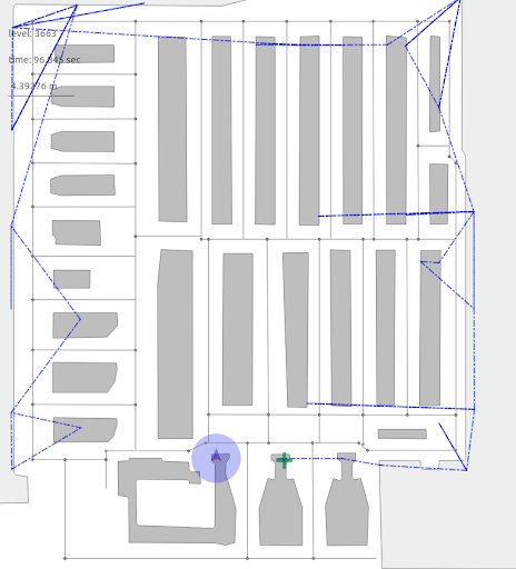
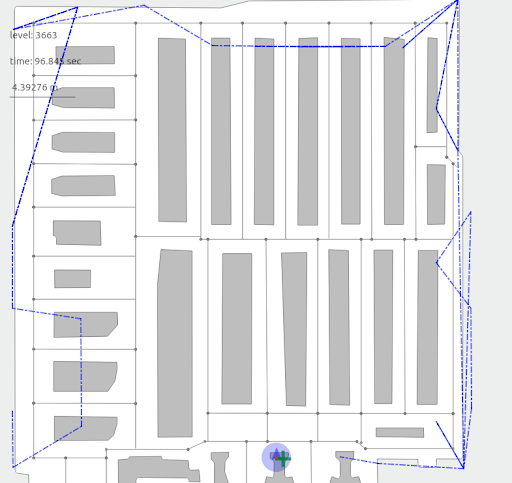
As you can see, the human position is discretized between points on the walls, while users are supposed to never walk near or through walls, but between them. Thus, the method gives us only an approximation of the user trajectory. If transmitters are placed evenly in the location space, by averaging them we will have the trajectory closer to the center of the corridor, which is closer to the true user motion trajectory.
The positive property of this method is that we see the transmitter we are mapped to in two ways: at the current time, and its expected position on the map. As a result, this method can be used if we are interested in testing beacons’ correct placement and configuration.
This algorithm on its own doesn't return us the perfect localization result. The trajectory is jumping between calculated discrete points. We can smooth the results using the implemented filter to create a more smooth and continuous pose progression.
If you are hooked by this article, rather go to our Github repository with positioning algorithms to learn more.